We have travelled from the Sea of Tranquility into the Sea of Rains. Now to the Northwest is our destination, the Bay of Rainbows.
The travel across the Sea of Rains is quite smooth, but our companions Peggy and Victor have been arguing all the way — arguing about the design of ZKP systems.
Victor: The trick with the cardboard was fun, but I'm not looking through a hole in some cardboard every time I want to check a proof.
Peggy: Of course not, we'll have a numeric representation of the proof.
Victor: It shouldn't be a lot of work to verify either. If it takes as long to verify as it takes to do the original computation, why have a proving system?
Peggy: True, we make it quick to verify.
Victor: And I don't want you telling me what to check. You might mislead me. I want to be able to check the proof however I like.
Peggy: OK, but don't think you are going to reverse engineer the proof and find my secret.
Victor: That's fair, but is this all possible? Will I need to learn some obscure and difficult mathematical objects to do this?
Peggy: Not at all. In fact, one of the major mathematical objects we will use is something you already know: the Polynomial.
We come over the final ridge into Sinus Iridum, The Bay of Rainbows. It is a massive, flat plain of basalt, but what catches the eye is the Montes Jura mountain range that curves around it.
In the low lunar light, the bay floor is in shadow, but the sun catches the peaks of the mountains, creating a perfect, glowing 'C' shape floating in the darkness. Astronomers call this the Golden Handle.
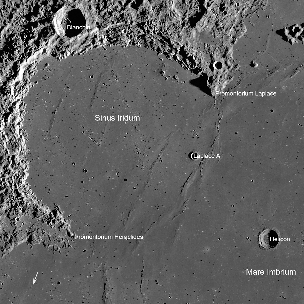
NASA, LRO — A Great Place to Rove!
Peggy points out the curve of the mountains to Victor.
"Look at that arc, that is a polynomial. On the ground, it's just a pile of scattered rocks, but from up here, you see the structure. You see the curve that connects them."
Polynomials
Fortunately for us, polynomials are straightforward, yet powerful mathematical objects that we have most likely some experience of from our schooldays.
A typical polynomial might look like:
$$y = 2x^3 + 4x^2 + 9x + 7$$
The polynomial is made of a number of terms added together, where a term is a variable to some power multiplied by a coefficient, such as $2x^3$.
The above is a univariate polynomial — we have just one variable $x$. But we can have multivariate polynomials that have more than one variable, such as:
$$z = 8x^2 + 3y + 4x + 9$$
Some of the properties of polynomials make them useful in ZKPs:
- Simple to manipulate: We can do arithmetic on polynomials quite simply.
- Dual Representation: They have two forms: a coefficient form (as above), or a point value form (where we list the points the polynomial passes through). There are simple means to convert between the two.
- Capacity: They can contain a lot of information; we can construct polynomials with millions of terms.
- Identity Testing: We can say with certainty and with minimal checking — even checking just one point — whether two polynomials are the same or different.
Let's dig into some of those points in more detail:
Point 2: The Two Views
If you imagine a polynomial plotted on a graph, we could describe it either by its equation (coefficients) or by the points it passes through.
- Coefficient Form: This is the "God's Eye View," like our Golden Handle. You see the whole curve as a single equation.
- Point Value Form: This is the view we get from the ground. On the ground, visiting specific coordinates, you don't see the curve; you just see "At mile marker 1, the altitude is 200m."
If we have the coefficients, we can easily calculate points. But what if we only have the points and want the curve? We can use a process called Lagrange Interpolation.
How Interpolation Works
How do we force a smooth curve to hit a random set of points? We use a technique that acts like building a mountain range. We don't build the whole curve at once; we build it point by point.
For every specific coordinate we want to hit (e.g., at $x=1$, height=5), we create a small mathematical 'ripple' that peaks exactly at that spot and is zero everywhere else. When we add all these ripples together, they combine to form one single, complex curve that fits every single point perfectly.
Point 4 is crucial to Victor's role
This seems impossible. How can checking just one coordinate tell you if an entire complex polynomial is correct?
This brings us to the Schwartz-Zippel Lemma, the mathematical bedrock of our journey. It relies on a simple geometric truth:
Different curves rarely touch.
Imagine two different polynomial curves winding across the Bay of Rainbows.
- They might cross each other once.
- They might cross twice.
- They might cross a thousand times.
But here is the key: The space they exist in (the Field) is vast — larger than the number of atoms in the universe. Compared to that vastness, even a thousand crossing points is nothing.
A Verifier's Test
Victor picks one random point $x$ from the entire universe of numbers. He asks Peggy to evaluate her polynomial at that point. He compares it to the evaluation of the expected polynomial.
- If the height (the y value) is different: The polynomials are definitely different. Peggy is cheating.
- If the height is the same: There are only two possibilities.
- A: The polynomials are identical everywhere. (Peggy is telling the truth).
- B: The polynomials are totally different, but Victor just happened to pick one of the tiny handful of points where they cross. (Peggy is lucky in the extreme).
Because the field of possible points is so huge, Possibility B is statistically impossible. Therefore, if the polynomials agree at just one random point, Victor can be overwhelmingly confident that they agree everywhere.
Victor is starting to realise that polynomials are going to be useful since they:
- Make it hard for Peggy to 'cheat' and convince him of an incorrect proof.
- Make his job of checking a proof relatively quick; testing a single point should tell him if two polynomials are different.
So if we could just reduce our ZKP system down to checking if two polynomials are the same, then Victor is going to be a happy verifier. However this is all getting a bit too hypothetical for him.
Victor: OK, let's take a concrete example. Imagine you have a password and I want to check that it contains more than 8 characters. You're not going to want to share your password with me. Can we do this with ZKPs?
Peggy: Yes, I could write a program that takes the password as an input and outputs "True" if it is the right length. However, we have to be careful what we are proving. I will make the claim that I ran the program against my password and got "True" as an output.
Victor: Would I be able to see the program code before you ran it?
Peggy: Indeed, there would have to be agreement between the prover and the verifier before we produce a proof, so that we both know what we are trying to prove and what the process is.
Victor: OK, so you run your program and it produces an output. If I want to absolutely be sure you didn't cheat, I would need to know that the program ran correctly, and applied the password length check. Will I have to check the program execution step by step?
Peggy: That would take too long, and anyway that might reveal the witness (the password I want to keep secret). We need a way to summarise the program execution in a way that still gives zero knowledge about the witness. That means taking our program execution details which we call the Execution Trace and going through a series of transformations. You can think of the Trace as the tracks left by the rover as we progress. We need to prove the track exists without showing the path we took.
Peggy: Polynomials are part of the overall process, but we need other maths also.
Victor: I thought we might.
Looking Ahead: The Problem of Precision
We have established that polynomials are the perfect vehicle for our proofs. But as we look out over the beautiful curves of the Bay of Rainbows, we hit an engineering problem.
In the real world, curves are smooth. To measure a smooth curve perfectly, you need infinite precision (using decimals that go on forever, like $\pi$). But computers are finite. They can't store infinite decimals. They need to apply rounding to numbers. In cryptography, rounding a number is fatal. If you are off by a tiny fraction of a decimal, the proof fails.
We need a world where we can have the complexity of curves but the exactness of integers. We need a world that doesn't stretch into infinity, but stays contained.
With this in mind we head West to the Oceanus Procellarum — the Ocean of Storms — to find a field where the horizon wraps around itself.